
Power Query For Data Preparation In Excel: An Introduction And Walk-Through For Beginners
November 2023
This article is rated as:


Introduction
If you’ve ever needed to analyze primary quantitative data yourself, you may know that a lot of the process is not spent on the analysis itself, but on preparing your data for analysis. Data preparation is the process of reworking your raw data into a useable format for your planned analysis, which is often time consuming, tedious, and prone to human error (especially if you have to repeat these steps on a recurring basis). If this is your first time preparing a dataset for analysis, check out some of our other helpful resources like ‘The Data Cleaning Toolbox’ and ‘Cleaning Messy Text with OpenRefine’ to learn more!
If you’re familiar with the data preparation process, then you know that it can be extra time consuming for recurring analyses where data is updated and needs to be re-analyzed for reporting at regular intervals. This is where Power Query, a tool designed specifically for data preparation integrated with Microsoft Excel, can be a game changer to your analysis workflow. Power Query lets you complete the data preparation task once while it records the steps you take so it can re-run automatically at the click of a button. In this article, I’ll guide you through my process of preparing a raw dataset for a recurring monthly analysis using Power Query and Excel and provide step-by-step instructions so you can try your hand at Power Query yourself.
To show you a little bit of what Power Query can do in helping you prepare your data, download this mock dataset and follow the steps below. If you’re using Excel 2016 or later, Power Query will be pre-installed. If you run into trouble accessing Power Query, check out some trouble shooting steps from Excel Campus here: https://www.excelcampus.com/install-power-query/
Below, I’ll walk you through different steps that I often take when setting up data prep queries. It is important to remember that the exact steps you take, and the order in which you take them, will vary depending on how your data is formatted and your own analytic goals! In this article, we’ll cover the topics listed under the Navigation menu.
(Tip: Click on any topic to jump to that section of the article!)
Navigation
- Exploring your data
- Loading data into Power Query
- Navigating the Power Query Editor
- Naming your queries
- Transforming your data
- Loading your data as a table
- Creating additional queries
- Refresh queries to auto-update analyses
Power Query Walk-Through
Open the downloaded file in Excel, and follow these steps to explore Power Query for the first time:
1. Exploring your data
If the video below is not loading, click here to open it in a separate tab.
When preparing for any analysis, it is important to explore your dataset to understand what types of variables you have to work with and create a plan. I created this small dataset to mimic a short survey that we might use to gauge the satisfaction of attendees of health-related programs across two Alberta cities. You will see that there are two worksheets in the file you have downloaded: data and new_data. For the first part of this tutorial, we will be working with only the data in the ‘data’ worksheet!

In the data worksheet, you’ll see that we have information about respondents’ demographics (age, gender), the program they attended (‘city_date’, ‘program_name’), their ratings of that program, and topics they would be interested in seeing in future program sessions (‘future_topics’). There are also two columns that contain meta-data, which is sometimes automatically collected by survey platforms (‘complete’, ‘responseID’).
There are a few key pieces of information that our clients have requested, which influences how I decide to prepare my data. Based on this, I plan to analyze the following pieces of information:
The demographic of survey respondents (age, gender)
The distribution of respondents over program types and sessions (program_name, city_date)
How respondents rated the program they attended, overall, by program type, and by session location
The most popular ‘future_topics’ among respondents, to inform the topic of our next session
My plan is to use Power Query to create two new tables from this data: one table of clean demographic, program, and rating data, and one table of future topics selected by respondents.
2. Load data to Power Query editor
If the video below is not loading, click here to open it in a separate tab.
There are tons of ways to load data to the Power Query editor, ranging from data within your active Workbook to external data saved on your device, in the cloud, or published online. To keep it simple, you’ll be loading data from the workbook. Start by formatting the dataset as a table (select the data range including headers then click ‘Insert’ > ‘Table’. Ensure ‘My table has headers’ is checked and click ‘OK’). It’s good practice to give your tables meaningful names, so let’s rename this table ‘t_raw’ in the ‘Table Name’ field of the Table Design ribbon up top.


Now that your data is in a table, click anywhere within the table and navigate to the ‘Data’ tab in the top ribbon. To the far left you should see a section called ‘Get & Transform Data’ – click ‘From Table/Range’ to load your table of data into the Power Query editor.

3. Navigating the Power Query editor
If the video below is not loading, click here to open it in a separate tab.
You should now have the Power Query editor open in a new window. There are six main sections in the Power Query editor that I’ll refer to throughout the next steps:
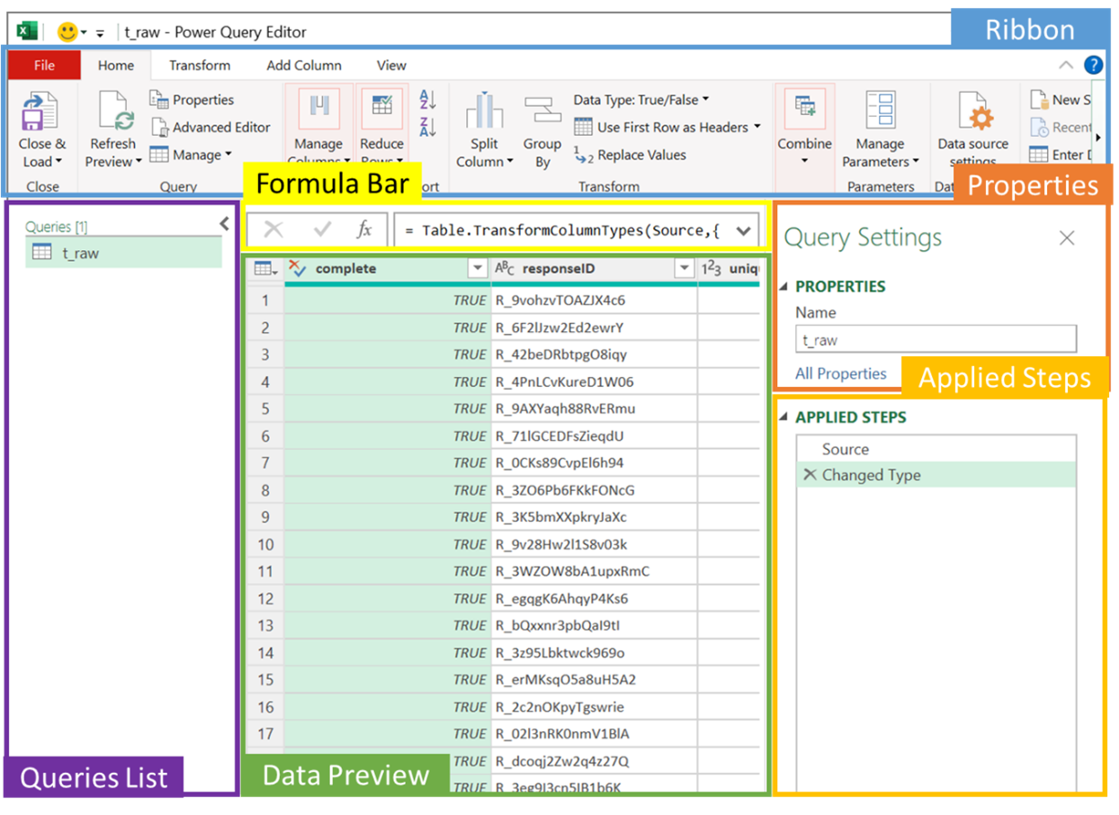
Ribbon: Like Excel, this ribbon contains command buttons organized across a few different tabs. For this tutorial, you’ll mostly be working in the Home and Transform tabs, but you might want to take a look through the Add Column and View tabs as well.
Queries List: This is where all the queries you’ve created within your file will be listed. Since this is your first query, there is just one in your list so far (but by the end of this walk-through there will be two).
Formula Bar: Power Query uses a formula language called M in the background to execute the transformations you will be applying to your data. Although Power Query displays this code, you don’t need to know how to code to use it! We won’t get into M code in this article, but if you’re interested in learning more, I’ve listed some great resources at the end of this article that you can check out.
Data Preview: As the name suggests, this section shows a preview of your data. This preview will change as you apply steps and is useful to make sure your transformations are working as you intended before you load your transformed data as a new table. The green bars below the column headers are useful in exploring your data, as they indicate missingness or errors within your variables. Hover over these bars to see detailed information about each variable!
Properties: Here is where you can rename your query, which is an important step in keeping your file easily manageable especially as you apply multiple queries.
Applied Steps: This is where Power Query records each transformation you apply as a ‘step’. You’ll notice two steps listed already, which were automatically applied by Power Query:
The ‘Source’ step refers to the data import from your data source, while the ‘Changed Type’ step refers to Power Query’s automatic transformation of data types based on the values within variables. You can click on the ‘Source’ step to see a preview of what the data looked like before Power Query applied the Changed Type step.
4. Naming your Query
If the video below is not loading, click here to open it in a separate tab.
Giving your query a meaningful name is one of the most important steps in keeping your file easy to manage (especially when working with multiple queries). The purpose of this query is to clean up your raw data into a table of clean data that you can use for analysis, so let’s rename this query ‘t_clean’.

5. Applying Transformations
As you’ve probably guessed by now, there are nearly infinite ways you can transform data in Power Query depending on the format of the raw data and the end goal of your data preparation. We’ll cover the basics using transformations directly in the Data Preview, as well as Transform and Add Columns tabs in this article.
5.1 Transformations in the Data Preview Section
5.1a Removing Variables
If the video below is not loading, click here to open it in a separate tab.
This dataset includes metadata which isn’t useful for your analysis. To remove these columns, simply hold ctrl (cmd on Mac) and click the column headers for the columns you want to remove, then right click and select ‘Remove Columns’.

You’ll notice that Power Query automatically added ‘Removed Columns’ to the list of Applied Steps – I like to rename my steps in case I need to make changes (especially when working on queries with many steps). To do this, right click on the step name, and select ‘Rename’, then specify a meaningful name for the step. Here, I’ll just add “metadata” to the step name to remind me of which columns I removed at this step.

5.1b Renaming Variables
If the video below is not loading, click here to open it in a separate tab.
Depending on the source of your data, your variable names may or may not be meaningful. In this case, your variable names do tell us something about the variable itself, but let’s rename the unique_id variable to make it shorter. Right-click on the column header and select ‘Rename’, then type in a new meaningful name for your variable. For this, I chose the name ‘ID’. Hit Enter or click away and Power Query will add an applied step – rename this step to indicate which column(s) was renamed in case you want to undo this in the future.
Note: You can also double-click on column headers, or use F2 with the column selected to rename your variables!

5.1c Changing Data Types
If the video below is not loading, click here to open it in a separate tab.
Power Query automatically updates data types based on the values within each column when it imports the data, but it doesn’t always get it perfect. I like to double check that each variable is assigned the correct data type, and update any that aren’t quite right. For example, Power Query saw that the variable ‘unique_id’ contained only numerical values and assigned it a numeric data type, which is indicated by the ‘123’ icon in the header of the unique_id header. Although it is right that these are numeric values, you won’t be treating them as numbers – you can change the data type of the unique_id variable to Text by clicking on the data type icon (the ‘123’ in the column header) and selecting ‘Text’ from the drop-down menu. By doing this, Excel will recognize these values as non-numeric, and will automatically count (instead of sum) these values when used in Pivot Tables.
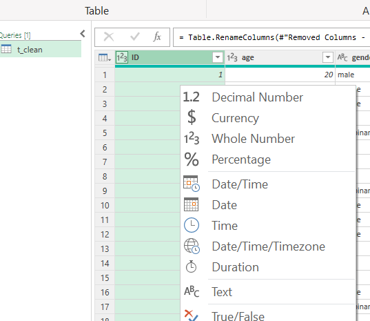
Remember to rename your Applied Step. I went with ‘Changed Type – ID to Text’
5.1d Reordering Variables
If the video below is not loading, click here to open it in a separate tab.
At this point, the data should be organized pretty well, with the ID variable to the far left, followed by demographics, program information, ratings, and future topics. In the case that youe wanted to reorganize variables, you could do so by simply clicking and holding down in the column header and dragging it to the desired location.

5.2 Transformations in the Transform Tab
5.2a Adding Prefixes
If the video below is not loading, click here to open it in a separate tab.
Even though you have now told Power Query to change the ID variable type to text, sometimes working with numeric values that are treated as non-numeric values can get confusing (especially towards the end of a long day!). I often like to add text values as prefixes to my ID values to prevent this by selecting the ID column, clicking ‘Format’ in the Transform ribbon, and choosing ‘Add Prefix’. Then I simply specify the text characters I want to add (here I went with ‘ID’) and click ‘OK’.

5.2b Capitalizing All Words
If the video below is not loading, click here to open it in a separate tab.
You may have noticed that the values in the gender and ratings variables are all in lower case. Although this doesn’t impact your analysis, it might be worthwhile to capitalize the beginning of each word to improve the look of the data if you will be sharing this file with clients or the public. To do this, select the column you want to reformat (hold ctrl or cmd to select multiple columns), then go to the ‘Transform’ tab in the ribbon and select ‘Format’, choosing ‘Capitalize Each Word’ from the drop-down menu.

5.2c Split Column by Delimiter
If the video below is not loading, click here to open it in a separate tab.
This is probably one of my most used basic transformations in Power Query as it allows us to separate a single column containing multiple pieces of data into multiple columns each containing one piece of data. In this case, you’ll use it to separate out the city_date variable into two columns, one containing the city the session was held in, and one containing the date of the session. Click on the city_date header to select the column, then click ‘Split Column’ under in the Transform tab of the ribbon, then choosing ‘By Delimiter’ from the drop-down menu.
Note: You can also find the ‘Split Column’ option in the Home tab.

‘Delimiter’ refers to the character or symbol that indicates the beginning or end of a data item. In this case, the delimiter is a hyphen surrounded by one space on each side. In the pop-up box that appears, Power Query likely recognized that a hyphen would be used as the delimiter automatically, but it didn’t include the space on either side of the hyphen. In this case, the left over spaces would live at the end of the city name and the beginning of the date value, which shouldn’t impact your analysis, but it is good to be aware of! To avoid any issues, I like to add a space on each side of the hyphen in the Split Column by Delimiter options window:

Click ‘OK’ – Power Query should have split your city_date column into two, which it automatically renamed city_date.1 and city_date.2 – let’s rename these to something meaningful (I went with ‘city’ and ‘session_date’) following the same process you used to rename your ID variable. You may have also noticed that Power Query automatically recognized the new session_date variable as a date and applied a Changed Type step automatically. Let’s update the names of your steps to something meaningful before moving on.
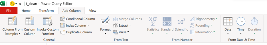
5.3 Transformations in the Add Column Tab
At this point, your data is pretty well prepped for the first table we planned, but let’s go one step further to explore some options in the Add Column tab.
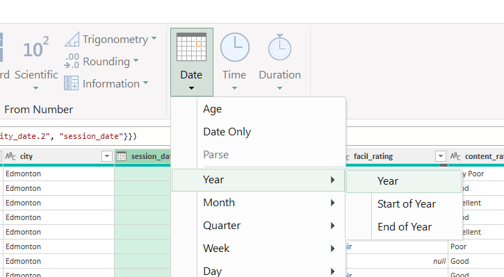
5.3a Adding Date Field Columns
If the video below is not loading, click here to open it in a separate tab.
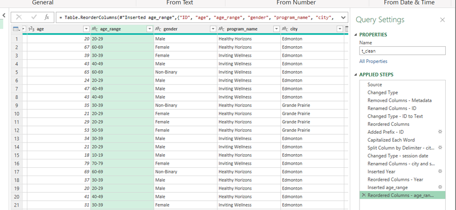
Maybe we are expecting to continue running sessions over the next 2 years and know that eventually, your client will want to see if respondents’ ratings of the sessions improve over that period. Although you could use the existing session_date variable, you might want to have a column that contains the year data only. You can do that by selecting the session_date column, then clicking ‘Date’ in the From Date & Time section to the far right of the Add Column ribbon and choosing ‘Year’ from the drop-down menu. You’ll notice that Power Query has added a column containing only the year data to the end of your data set. Let’s click and drag to move the Year variable next to the session_date variable.
5.3c Adding Columns From Examples
If the video below is not loading, click here to open it in a separate tab.
Another super useful option in the ‘Add Columns’ ribbon is ‘Column From Examples’, which allows us to show Power Query examples of values that you want in a new column based on an existing column, and lets it fill in the rest automatically. Let’s test this out by creating an age range variable based on the respondent’s age. Select the age column header, then click on the drop-down arrow for ‘Column From Examples’ in the far left of the Add Column ribbon and choosing ‘From Selection’. Now you should see a blank column in the right of the Data Preview section with the age column header highlighted in green. I first entered 20-29 in the new column for row 1, which Power Query interpreted as creating a 9-year age range starting from the specified age, which isn’t exactly what I wanted.
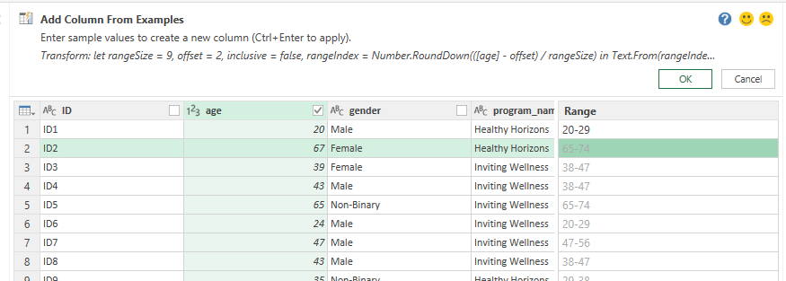
The more examples you provide, the better Power Query will be able to auto-fill the remaining rows, so I typed in 60-69 in the next row. This was enough information for Power Query to auto-fill the rest of the rows with the age ranges I was looking for!

Update the column name by double-clicking in the column header and entering ‘age_range’, then click OK. You now have an age_range column at the end of your data set – click and drag it to beside the age variable, then rename your steps.
Note: You can name variables using any convention that you like. I prefer to separate multi-word variables using underscores to maintain consistency across my work, but do whatever works best for you and your organization!
6. Close & Load To…
If the video below is not loading, click here to open it in a separate tab.
Our data for the first clean table we planned is ready! To submit this query and load your clean data into a table within your Excel workbook, go to the Home tab of the ribbon, select the ‘Close & Load’ drop-down menu, and choose “Close & Load To…”.

A pop-up window will open asking how you want to view this data, and where you want to put it in your workbook. In this case, you will want to view it as a table, and add it to a new worksheet, so leave the selections as they are and press OK.

You should now have a new table containing the transformed data in a new worksheet that is ready to be summarized in Pivot Tables.
7. Creating Additional Queries
If the video below is not loading, click here to open it in a separate tab.
We still need to analyze the most commonly selected topics among respondents for future sessions, which is something we didn’t prepare for in our first query. Although you could probably make this work all within one query, it would add lots of extra steps and likely involve some coding in M to achieve. Instead, I find it easier to create a separate table for this type of data, where each selected topic selected by a respondent is listed in a separate row along with its corresponding ID value, program name and session location. This makes it a breeze to analyze using Pivot Tables!
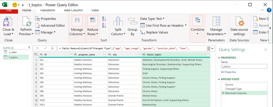
To create a new query, repeat ‘Step 2. Load data to the Power Query editor’ from above, this time using the table you just created (t_clean) as the source. Rename this new query to t_topics to remind you that this query is used to create your topics table.
Hint: If you’re not sure how to use your t_clean table as the source for your new query, simply click anywhere within the t_clean table, then select ‘From Table/Range’ in the ‘Get & Transform Data’ section of the ‘Data’ tab!
7.1 Remove Unnecessary Variables
If the video below is not loading, click here to open it in a separate tab.
Since you have the data you need for the first few analysis goals in your t_clean table, you don’t need them to also appear in your t_topics table. Using Power Query, remove all the columns except for ID, program_name, city, and future_topics.
7.2 Split Column by Delimiter
If the video below is not loading, click here to open it in a separate tab.
Now, let’s split the future_topics column by a delimiter. Power Query should recognize that the delimiter you’ll be using is a comma, but you can change this to ‘Custom’ and type in a comma followed by a space if you want to save yourself a step down the line. Since there can be more than one delimiter in this column, and you want each selected topic to be in its own column (which you will soon turn into rows), double check that ‘Each Occurrence of The Delimiter’ is selected, and then click OK.

You should now have four new columns in place of the future_topics column. Note that the number of columns created will depend on the maximum number of delimiters within the variable.
If you chose to enter a comma followed by a space as a custom delimiter in the last step, you can move on to Unpivoting Columns. Otherwise, you may want to remove the spaces that now live at the beginning of each selected topic value after the first. To do this, hold ctrl (or cmd on Mac) and click to select future_topics.2, future_topics.3, and future_topics.4 columns, then click ‘Format’ in the Transform ribbon and select ‘Trim’ from the drop-down menu. This tells Power Query to remove any unnecessary spaces at the beginning or end of character strings to keep your data tidy and consistent.
7.4 Unpivoting Columns
If the video below is not loading, click here to open it in a separate tab.
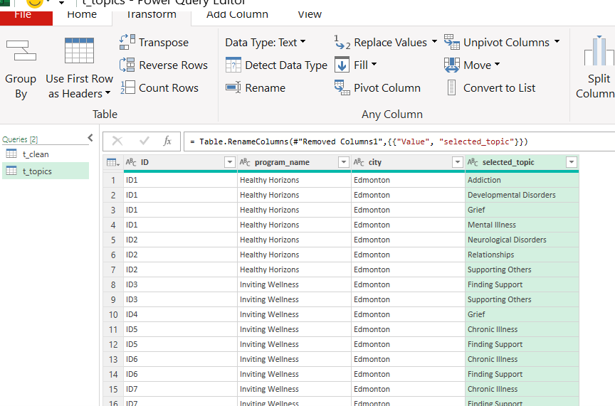
Now you can transform your wide data set (which has many columns and just one row per respondent) into a long data set (where there are many rows and fewer columns per respondent). You only want to unpivot the topics columns, so hold ctrl (cmd on Mac) and click to select each of the future_topics columns, then click the drop-down arrow beside ‘Unpivot Columns’ in the Transform ribbon and choose ‘Unpivot only selected columns’.

Now you can see that each respondent has multiple rows, but just two columns for their selected topics (compared to the four you had after splitting). In this case, it’s not important to know the order that topics were selected in, so the Attributes column is not needed. Let’s remove it, and then rename the ‘Value’ column to ‘selected_topic’.
Now your data is ready to be analyzed to determine the most commonly selected topic overall, by program name, and by location. Let’s close and load this data as a table to a new worksheet, following ‘Step 6. Close & Load To…’ from above.
8. Using Power Query to easily update analyses with new or updated data
If the video below does not load, click here to open the video in a separate tab.
Using your new t_topics table, you can now use Pivot Tables (check out our Pivot Table article here!) to analyze the most popular topics for future sessions among respondents overall, and broken down by program name.
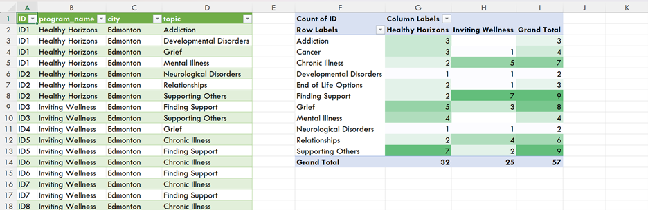
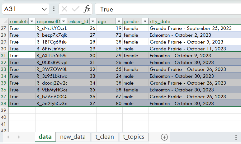
The best part about Power Query is that once you’ve applied all the transformations you need to get your data prepared for your analysis, when new data is added to the data set, you can simply hit ‘Refresh All’ in the Data tab of Excel, and Power Query will automatically apply the transformations to your new data saving you time when working on recurring analyses! Let’s test this out by copying the data from the new_data worksheet into your t_raw table in the data worksheet, then clicking ‘Refresh All’ in the Data tab of the Excel ribbon.
Copy data (excluding headers) from the new_data worksheet by selecting it and using ctrl + c (or cmd + c on Mac) to copy the new data…

… and ctrl + v (or cmd + v on Mac) to paste it in the first row below your original raw data table.
Next, select the table you want to update, navigate to the Data tab ribbon, click ‘Refresh All’ and watch Power Query work its magic! Your table should update with the new data values formatted according to the steps you applied in the Query connected to the table.

Repeat this ‘Refresh All’ step for each queried table in your workbook. As long as your new data is in the same format each time, Power Query will be able to apply all the steps you’ve specified across all your queries with just one click, and seamlessly update any connected Pivot Tables or formulae you may have applied in your workbook!
Before refreshing with new data:

After data refreshing with new data:

Now that you’ve had some practice applying basic transformations using Power Query and Microsoft Excel, you’re ready explore the hundreds of other options available in Power Query in your own data preparation tasks!
M Programming Language Resources:
Interested in applying more advanced queries using M in Power Query? Check out these M Language resources:
Quick tour of the Power Query M formula language by Microsoft:
https://learn.microsoft.com/en-us/powerquery-m/quick-tour-of-the-power-query-m-formula-languagePower Query M Formula Language Guide by Microsoft:
https://learn.microsoft.com/en-us/powerquery-m/Basics of M: Power Query Formula Language by RADACAD:
https://radacad.com/basics-of-m-power-query-formula-languageFree M Code Class from Basic to Advanced: Power Query Excel & Power BI, Custom Functions 365 MEC 12 by ExcelIsFun on YouTube: https://www.youtube.com/watch?v=3ZkIwKBVkVE